Apr 20, 2024 16:00:00

What is the mechanism behind 'Vision Transformers,' a machine learning model developed by Google that can perform image classification tasks?

Google's machine learning model '

Transformer ' can translate and summarize natural language and other data without processing the data chronologically, and is the basis of chat AI that can have natural conversations, such as ChatGPT. In addition, ' Vision Transformer ' is a model that applies Transformer's techniques to the image field. Software engineer Dennis Tharp provides a visualization of how the components of 'Vision Transformer' work and how the data flows.

A Visual Guide to Vision Transformers | MDTURP
https://blog.mdturp.ch/posts/2024-04-05-visual_guide_to_vision_transformer.html

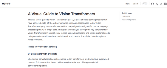
0: Introduction
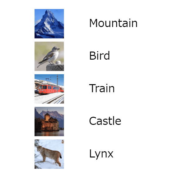
First, similar to how the Transformer works, the Vision Transformer is supervised, meaning the model is trained on a dataset of images and their corresponding labels.

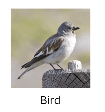
1: Focus on one piece of data
We pick up a single piece of data called 'patch size 1'.

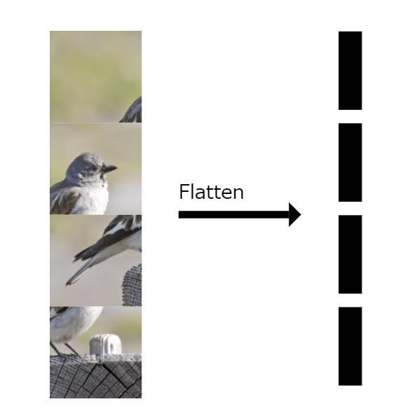
2: Image division
To make an image usable by the Vision Transformer, we divide the image into equal-sized patches.

3: Flattening image patches
Convert the patch into a vector of p' = p²*c, where p is the size of the patch and c is the number of patches it is split into.

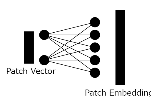
4: Creating patch embedding vectors
(PDF file) Using

a linear transformation , the image patches converted into vectors are further converted into patch embedding vectors.

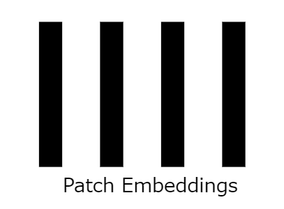
5: Apply to all patches
We convert all patches into patch embedding vectors, which results in an nxd array, where n is the number of image patches and d is the size of the patch embedding vector.

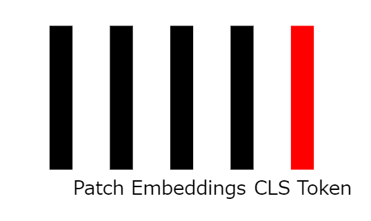
6: Adding classification tokens
To effectively train the model, we add a vector called the classification token (cls token), which is a learnable parameter of the network and is initialized randomly.

7: Adding position embedding vectors
Up until now, the vectors have no location information associated with them, so we add a learnable, randomly initialized 'location embedding vector' to all vectors, including the cls token.

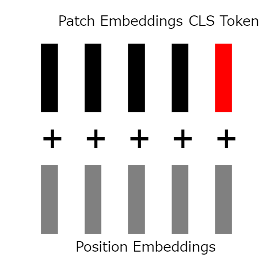
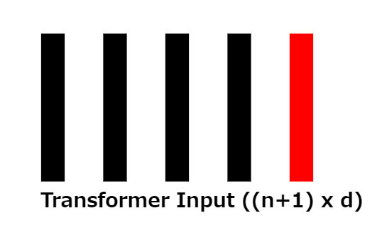
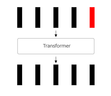
8: Transformer input
Once the position embedding vectors are added, we are left with an array of size (n+1) × d, which corresponds to the input to the transformer.

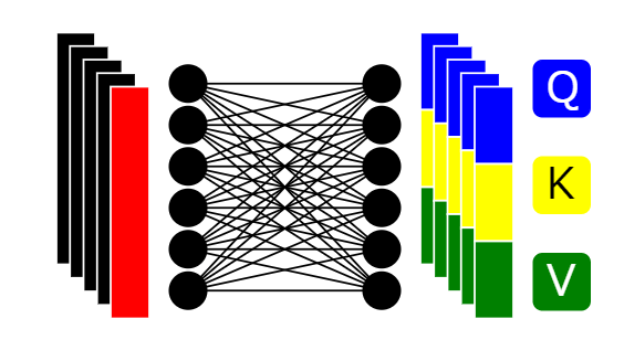
9: Allocation to three types of vectors
The array of size (n+1) × d is divided into a 'query vector' corresponding to Q, a 'key vector' corresponding to K, and a 'value vector' corresponding to V.

10: Calculating Attention Score
To compute the attention score, we multiply every query vector by the key vector.

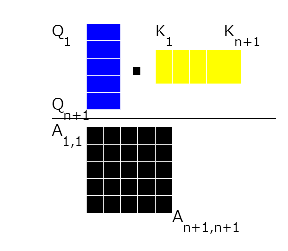
11: Attention score matrix
Now that we have the attention matrix from the calculations, we apply the “

Softmax ” function to every row so that the sum of all rows is 1.

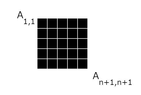
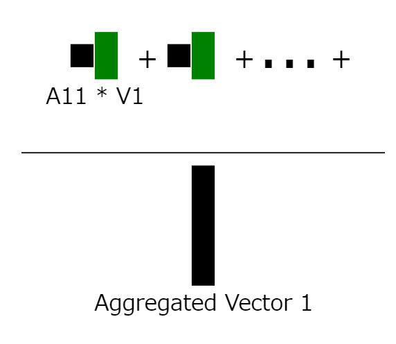
12: Calculating aggregated context information
We focus on the first row of the matrix and calculate the aggregated context information of the patch embedding vector, then use the whole as the weight of the value vector to obtain the aggregated context information vector of the first patch embedding vector.

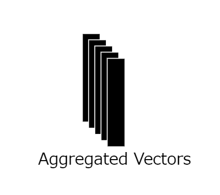
13: Apply to all rows
We apply this calculation to the entire attention matrix, resulting in N+1 aggregated context information vectors.

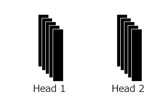
14: Repeat the process
This process is repeated multiple times depending on the number of

heads , resulting in multiple aggregated context information vectors being output.

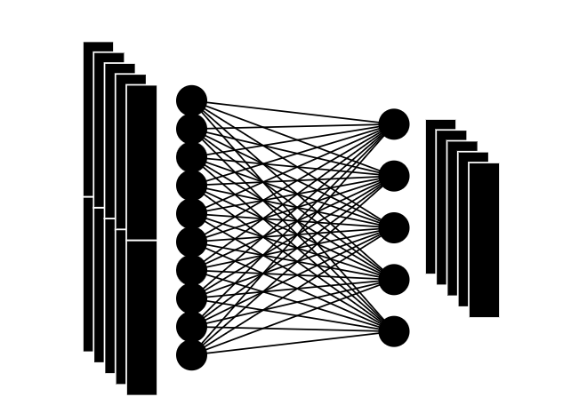
15: Mapping to a vector of size d
We merge multiple heads and map them into a vector of size d, the same as the patch embedding vector.

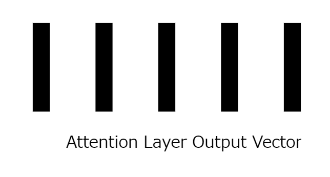
16: Completion of attention layer
The mapping to a vector results in an embedding that is exactly the same size and quantity as the input embedding vector.

17: Application of residual connections
The input of the layer that adds the position embedding vector is added to the output of the attention layer.

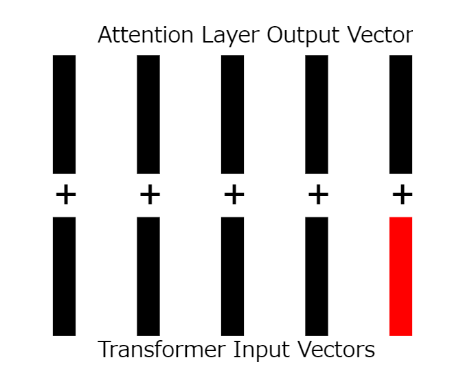
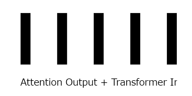
18: Calculate the remaining connections
Add the inputs and outputs together.

19: Feedforward network
The outputs generated so far are fed through

a feedforward network with a nonlinear activation function.

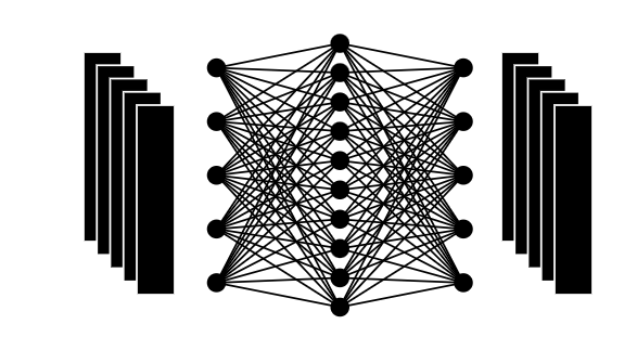
20: Final result
By performing multiple operations, an output of the same size as the input was produced.

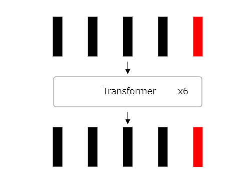
21: Repeat the process
Repeat this process multiple times.

22: Identifying classification token output
The final step in Vision Transformer is to identify the classification token outputs.

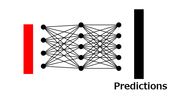
23: Classification probability prediction
We use the output of the classification tokens and another fully connected neural network to predict the classification probability of the original image.

24: Vision Transformer training
We train a Vision Transformer using cross-entropy error .