Nov 02, 2020 09:15:00

What happens when Bayesian inference is incorporated into 'Q-learning' of machine learning?

'

Q-learning, ' which is a type of reinforcement learning in machine learning, is a method in which an agent who is the main actor learns the optimal answer from the current situation, the future situation, and the rewards obtained. Machine learning engineer Brandon Da Silva is conducting research that incorporates Bayesian inference elements into such Q-learning.

brandinho.github.io/bayesian-perspective-q-learning/
https://brandinho.github.io/bayesian-perspective-q-learning/

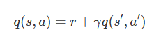
The basic idea of Q-learning is that 'the value of a certain state (Q value) is determined by the reward obtained and the value of the state at the next point in time', and is expressed by the following formula. 'Q (s, a)' is the value when an action is taken from the current state, 'r' is the reward obtained, and 'q (s', a')' is the action from the state at the next point. It represents the value at the time of taking, and 'γ' represents the discount rate that discounts the value of the next point to the current value.

In actual Q-learning, the Q value also depends on the learning rate indicated by 'α'. The learning rate is the degree of influence of new information on learning, and is a hyperparameter that is fixed in advance. The Q-learning formula including the learning rate is as follows.

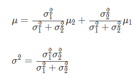
The composition of Q-learning, 'update the current information based on new information,' is very similar to Bayesian estimation . Assuming that the Q value follows a normal distribution , the above formula can be applied to the formula for finding posterior probabilities in Bayesian estimation. The mean μ and variance σ ^ 2 of the posterior distribution can be expressed by the following equations.

Comparing the Q-value formula with the formula for averaging the posterior distribution in Bayesian estimation, we can see that in Q-learning, α, that is, the learning rate is a hyperparameter, so the yellow and purple values are fixed values. Mr. Silva explained that Q-learning can be regarded as an operation to update posterior probabilities only by average in Bayesian estimation.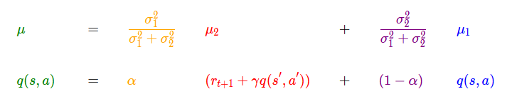

It looks like this when you visualize how the information is updated about the normal Bayesian estimation and the Bayesian estimation with α fixed. With α as 0.5, the first starting point is the same for both.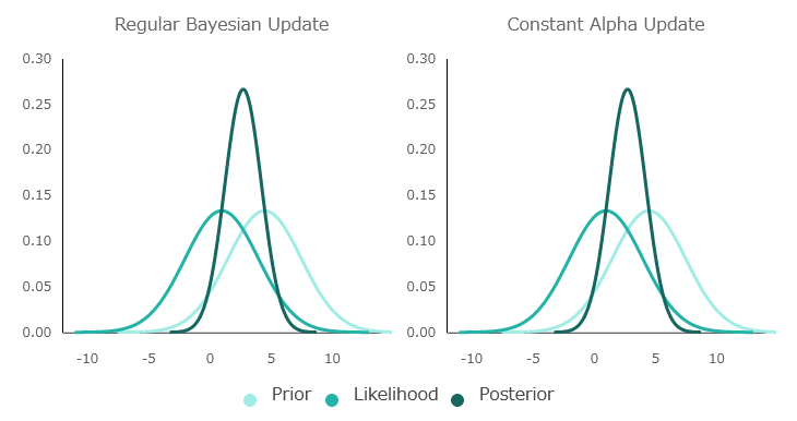

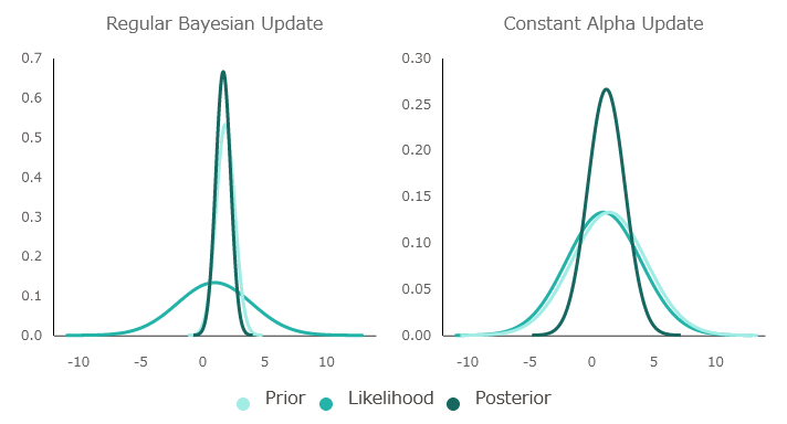
In normal Bayesian inference, information is updated efficiently by manipulating the value of α and giving priority to the 'current information', but when α is fixed, new information and old information are treated equally, so the information is updated. Will be delayed.

The difference grows steadily as you learn more. In other words, Silva's opinion is that Q-learning can be learned faster by dynamically changing the learning rate in the same way as Bayesian estimation. Even in actual Q-learning research, there is a method to reduce the learning rate with each learning. By incorporating the elements of Bayesian inference into Q-learning, agents will act while flexibly changing 'whether they value current information or new information' as they learn.

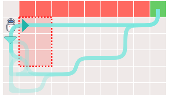
Q Silva prepares a game using an agent so that you can experience learning. The field of the game is divided into 'goal', 'cliff', 'danger zone', and 'roaming state', and the rewards are '50' for the goal, '-50' for the cliff, and '-15' for the dangerous zone. The probability distribution of '1' and the roaming state are the probability distribution of the expected value '-2'.

First, set the number of learning times to '40' and click 'Play'.

The agent has started working.

The green squares have a high Q value, and the red squares have a low Q value. The agent has a Q value for each direction to go to the square, and when acting, it goes to the square with the higher Q value.

When the number of learnings was 40, it timed out and I could not reach the goal.

When I learned 5000 times, I was able to reach the goal safely. The more you learn, the more you can observe the agent progressing to the goal without hesitation.

In Q-learning using Bayesian estimation, if the number of learnings is large enough, the agent can find the way to the goal without falling off the cliff.

However, there are problems with Q-learning using Bayesian inference, Silva explained. Originally, the green route is the optimum route, but depending on the situation, it seems that you may learn the non-optimal route through the danger zone (red in the figure below).

It is said that this phenomenon occurs when the agent cannot search for the optimum route before the Q value diverges. Silva explains that learning stops when the Q factor diverges, so we need to find the best route before that.

Let's take a closer look at the behavior of the agent who learned the suboptimal route. If the Q value diverges before searching for the optimal route, the agent will not learn the 'bottom' route, which has a higher Q value than the 'right'.

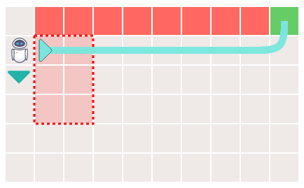
If you force the agent to move 'down' here, you will find that you may avoid the danger zone and reach the goal. For this reason, Silva explained that forcing the agent to move to the optimal route helps to separate the 'bad memories' that the agent has learned in the past and select the optimal route. I am.

Silva concludes his attempt to incorporate Bayesian inference into Q-learning, pointing out that while theoretically great, it can be difficult to apply in a real environment. However, he commented that the research field itself is exciting and he expects cutting-edge research.