Mar 21, 2026 12:00:00

Lessons learned from a 4-month image and video VAE experiment with generative AI.

While video generation technology has made remarkable progress, designing and training the underlying

VAE (Variational Autoencoder) still presents many challenges. Linum , an AI lab, has detailed the challenges they faced and the valuable insights they gained while developing a VAE that supports both images and videos in their company blog.

Better Reconstruction ≠ Better Generation | Field Notes by Linum
https://www.linum.ai/field-notes/vae-reconstruction-vs-generation

While

diffusion transformers are the dominant method in video generation, their computational cost is enormous, making direct processing in pixel space impractical. For example, to shoot a 5-second video at 24fps with a resolution of 720x1280px, processing in pixel space would require the following amount of data, based on simple calculations.
$$720 \times 1280 \times 5 \times 24 = 110{,}592{,}000 \text{raw pixels}$$ Processing 110 million tokens in a very short video is absurd, so the role of VAEs, which can compress videos into a more compact latent space , becomes essential. The purpose of an autoencoder is to capture the essential features of data by 'compressing the input data with an encoder' and 'reconstructing the original data with a decoder,' but the characteristic of a VAE, a type of autoencoder, is that the encoder outputs a probability distribution of $z$ as a parameter, rather than a single point $z$, and by utilizing the output of the VAE, sampling from the latent space becomes possible.

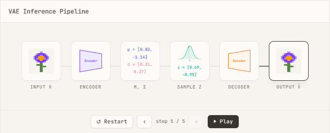
The actual calculation involves passing the data sample $x$ through an encoder to determine the mean and standard deviation for each latent dimension, thereby defining

a multivariate Gaussian distribution . Then, the reconstructed value $\hat{x}$ is obtained by sampling $z$ from the multivariate Gaussian distribution and decoding it. Therefore, training a VAE means minimizing the following loss.
$$\mathcal{L}_{\text{modality}} = \lambda_1 \cdot \mathcal{L}_{\text{KL}} + \lambda_2 \cdot \mathcal{L}_{\text{recon}} + \lambda_3 \cdot \mathcal{L}_{\text{perceptual}} + \lambda_4 \cdot \mathcal{L}_{\text{adversarial}}$$
• $\mathcal{L}_{\text{KL}}$: KL divergence between the probability distribution of the latent variable $z$ and the normal distribution (approaching the latent distribution to a simple distribution)
• $\mathcal{L}_{\text{recon}}$: Reconstruction loss (minimizes the difference between the original data and the reconstructed data)
• $\mathcal{L}_{\text{perceptual}}$: Perceptual loss (minimizing the perceptual difference between the reconstructed data and the original data)
• $\mathcal{L}_{\text{adversarial}}$: Adversarial loss (makes the generator appear real)

Linum initially began by building a VAE (Video-Aided Engineering) specifically for video, employing a convolutional neural network (CNN) -based encoder-decoder architecture.

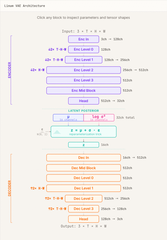
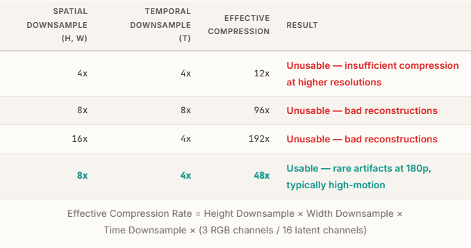
To find the optimal memory usage, we started with 4x spatial and 4x temporal compression, and then experimented with higher compression ratios. The results showed that a practical level could be achieved with 8x spatial and 4x temporal compression (a total of 48x compression).

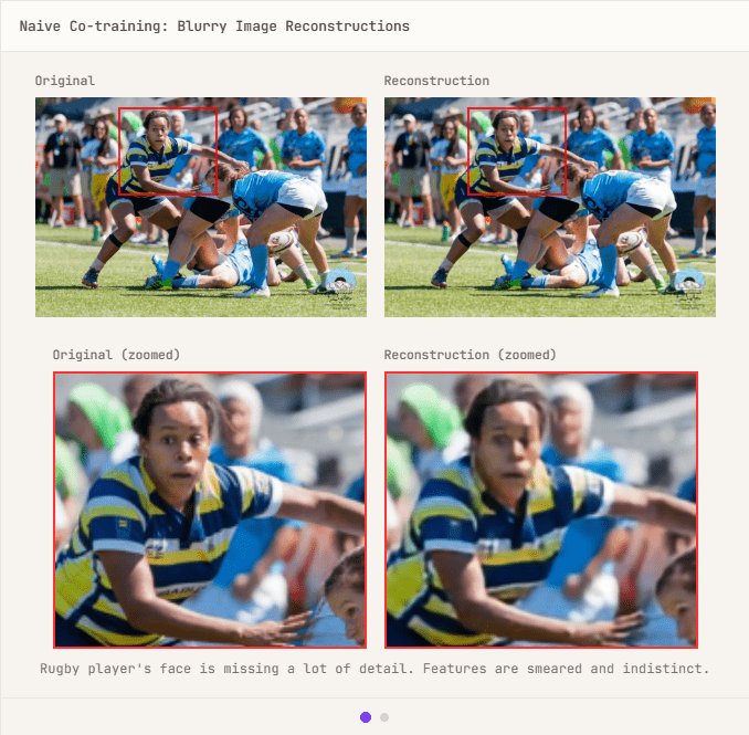
While the VAE development process for video-only models went very smoothly, taking only one week, the inclusion of still images resulted in a problem of 'deterioration in image reconstruction quality.'

First, considering the possibility that the 'still image' approach to image reconstruction might be unstable, we retrained the network using only still images. This resulted in performance equivalent to that of a VAE using only video. Therefore, we decided to investigate the loss function in detail to find the reason why the reconstruction results deteriorate when training with 'still images + video'. The standard form for dividing the sum of reconstruction losses for all dimensions ($C × T × H × W$) by the batch size ($B$) is as follows.
By examining the above equation, we found that there is a problem in that the 'magnitude of the loss' is

proportional to the tensor size. The reason why this proportionality to the tensor size is a problem is that the tensor size differs greatly between still images and videos. A simple correction would be to apply the following standard formula, which obtains the average value for each sample.
$$\mathcal{L}_{\text{recon}} = \frac{1}{B} \sum_{i=1}^{B} \frac{1}{C \cdot T \cdot H \cdot W} \sum_{c,t,h,w} \text{NLL}(x_i, \hat{x}_i)$$ However, this time the gradient per pixel becomes inversely proportional to the tensor size, which would place an excessive emphasis on the reconstruction of still images. As a solution, relative normalization with respect to the reference shape ($S_{\text{ref}}$) was introduced.
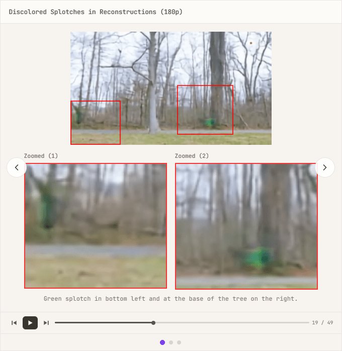
$$\text{scale} = \frac{|S_{\text{ref}}|}{C \cdot T \cdot H \cdot W}$$ $$\mathcal{L}_{\text{recon}} = \text{scale} \cdot \frac{1}{B} \sum_{i=1}^{B} \sum_{c,t,h,w} \text{NLL}(x_i, \hat{x}_i)$$By applying the above equation, we were able to re-evaluate the importance of different resolutions and modalities while keeping the magnitude of the loss constant regardless of the resolution. However, when we tried applying the same weighting to still images and videos, we encountered a problem that Linum calls 'NaN hell,' where the calculation result becomes NaN . Initially, we suspected the issue was due to the model having difficulty distinguishing between still images and videos, so we tried introducing a FiLM (Feature-wise Linear Modulation) layer as a countermeasure, but it had no effect. Giving up on the proper approach, we introduced Adaptive Gradient Clipping (AGC) as a 'hack' to stabilize training, and training became stable. However, this time, discolored spots started appearing in the reconstructed images.

Upon investigating whether similar cases had been reported in the past, we found that

the developers of LiteVAE had faced a similar problem , so we decided to implement their solution , Self-Modulated Convolution (SMC) . SMC is a technique that normalizes the 'convolution weights' instead of output activation, and each weight is scaled by a parameter $s_i$ learned for each input channel, allowing us to control how much each input channel contributes to the output.
$$w'_{ijk} = \frac{s_i \cdot w_{ijk}}{\sqrt{\sum_{i,k}(s_i \cdot w_{ijk})^2 + \epsilon}}$$SMC allows the network to modulate each channel independently and prevents abnormal increases in activation, enabling the model to handle large amplitude signals more flexibly and thus helping to avoid the occurrence of spots. After three months of trial and error, the VAE was working correctly, but it had been optimized for 720px data, the final checkpoint, neglecting the reconstruction of low-resolution images and videos, so we spent another two weeks training on data of various resolutions simultaneously.

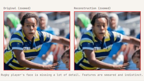
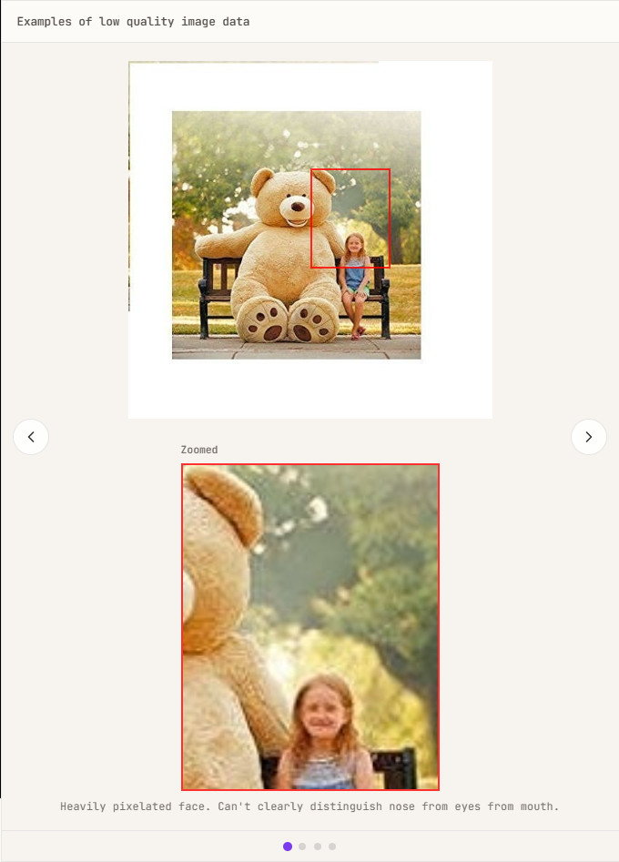
Initially, Linum aimed to perfectly reconstruct images pixel by pixel during the process of building VAEs. However, as research progressed, it became clear that high reconstruction quality does not necessarily lead to improved generation quality in downstream diffusion models. For example, using low-quality image data, such as that with excessive JPEG compression, can result in it being perceived as noise, making it more difficult to reconstruct than actual detail. Trying to force a perfect reconstruction with a VAE distorts the latent space in an attempt to capture detail. In other words, excessive focus on reconstruction quality can lead to a VAE simply spewing out noise.

It was discovered that the high instability of simultaneous learning across resolutions was due to an overemphasis on reconstruction quality. This led to the realization that VAEs that perform higher-quality reconstructions may generate inferior diffusion models, potentially impairing the diffusion model's ability to learn visual concepts. Linum's blog states that a key lesson learned from this four-month experiment is that pursuing reconstruction quality does not necessarily lead to improved generation quality .